Build Your First Neural Network from Scratch (Step-by-Step Tutorial)

Ever wondered how machines “learn” to recognize faces, drive cars, or even write text? At the core of all that intelligence lies something called an Artificial Neural Network (ANN).

And today, we’re not just going to talk about neural networks – we’re going to build one completely from scratch using Python and NumPy. No TensorFlow, no PyTorch – just the pure logic that powers machine learning.

---

What Is a Neural Network?

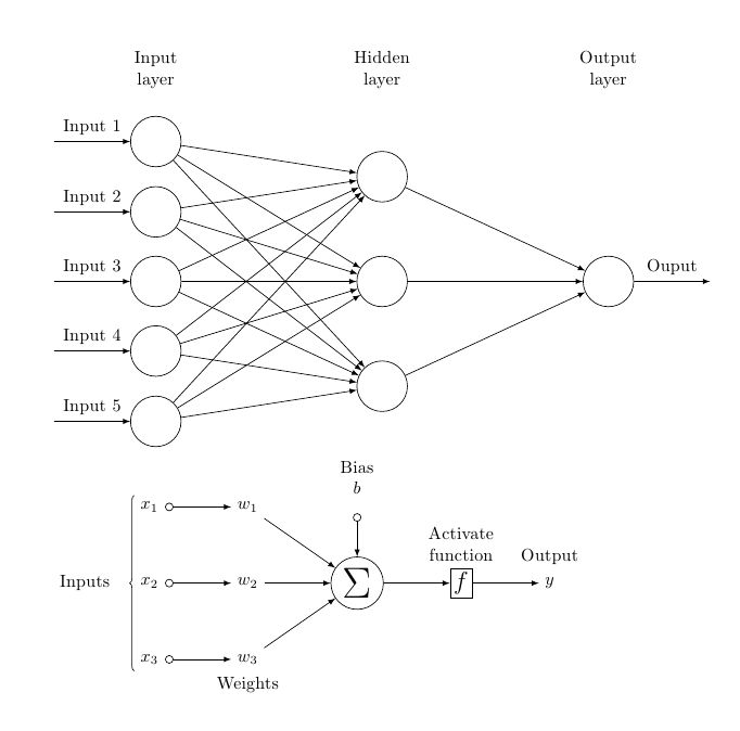
A neural network is inspired by how the human brain works. It’s made of interconnected “neurons,” each taking in inputs, applying weights, adding bias, and sending the result through an activation function.

When a network predicts something incorrectly, it adjusts its weights – little by little – until it learns the correct patterns. This process is called learning.

Think of it like teaching a kid to recognize cats. At first, they guess wrong, but after seeing enough examples, they just get it. Neural networks do the same thing, only using math instead of words.

---

How Neural Networks Learn — The Intuition

Before writing a single line of code, let’s understand what’s happening behind the scenes.

Neural networks learn by minimizing a loss function — a number that tells how “wrong” the network is. Each time it makes a guess, it measures that loss and adjusts the weights slightly to reduce the error.

This adjustment process is called gradient descent. You can imagine it as rolling down a hill, taking small steps until you reach the lowest point – the minimum loss.

In simple terms, the network keeps repeating this cycle:

• Start with random weights.
• Make a prediction.
• Measure how wrong it was (loss).
• Adjust the weights.
• Repeat many times until it learns.

---

Building a Neural Network Step by Step

We’ll build a simple neural network that learns the XOR pattern – one of the classic examples in AI.

Step 1: Import Libraries

import numpy as np
import matplotlib.pyplot as plt

We’re keeping things lightweight – only NumPy for the math operations.

---

Step 2: Create the Dataset

X = np.array([[0,0],
              [0,1],
              [1,0],
              [1,1]])

y = np.array([[0],
              [1],
              [1],
              [0]])

This is our XOR dataset. The output is 1 only when one input is 1, not both.

Input 1	Input 2	Output (y)
0	0	0
0	1	1
1	0	1
1	1	0

---

Step 3: Initialize Parameters

np.random.seed(42)

W1 = np.random.randn(2, 2)
b1 = np.zeros((1, 2))
W2 = np.random.randn(2, 1)
b2 = np.zeros((1, 1))

We’re defining:

• 2 input features
• 2 neurons in the hidden layer
• 1 output neuron

Weights (W) start as random numbers, and biases (b) start at zero.

---

Step 4: Define the Activation Function

def sigmoid(x):
    return 1 / (1 + np.exp(-x))

def sigmoid_derivative(x):
    return x * (1 - x)

The sigmoid function squashes numbers between 0 and 1, making it ideal for probabilities.

---

Step 5: Train the Neural Network

lr = 0.1  # learning rate
epochs = 10000
loss_history = []

for epoch in range(epochs):
    # Forward pass
    z1 = np.dot(X, W1) + b1
    a1 = sigmoid(z1)
    z2 = np.dot(a1, W2) + b2
    output = sigmoid(z2)

    # Calculate loss
    error = y - final_output
    loss = np.mean(np.square(error))
    loss_history.append(loss)

    # Backward pass
    d_output = (y - output) * sigmoid_derivative(output)
    d_hidden = np.dot(d_output, W2.T) * sigmoid_derivative(a1)

    # Update weights and biases
    W2 += np.dot(a1.T, d_output) * lr
    b2 += np.sum(d_output, axis=0, keepdims=True) * lr
    W1 += np.dot(X.T, d_hidden) * lr
    b1 += np.sum(d_hidden, axis=0, keepdims=True) * lr

    if epoch % 1000 == 0:
        print(f'Epoch {epoch} Loss: {loss:.4f}')

Here’s what’s happening step-by-step:

• Forward pass: The network makes a prediction.
• Loss calculation: Measures how wrong it is.
• Backward pass: Adjusts weights to improve the next prediction.
• Learning rate (lr): Controls how big each step is during learning.

---

Step 6: Test the Network

print("Predictions:")
print(output.round())

After training, you’ll get outputs close to [0, 1, 1, 0] — meaning your little neural network has successfully learned XOR! 🎉

---

Understanding What’s Happening in the Code

Let’s quickly recap what’s really going on inside the network:

• Forward Pass: Each neuron multiplies inputs by weights, adds bias, and applies the activation function. This produces an output.
• Backward Pass: The network checks how far off its predictions were, then updates weights to reduce future errors. This is called backpropagation.
• Epochs: One full cycle of training (forward + backward). The more epochs, the better it learns – up to a limit.

---

Experiment & Play

Now that it’s working, don’t stop here! Try making small tweaks:

• Change the learning rate to see how it affects convergence speed.
• Add more hidden neurons or even an extra layer.
• Swap the activation function for ReLU or tanh.

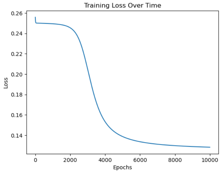
You can also visualize training with a loss curve:

import matplotlib.pyplot as plt
plt.plot(loss_history)
plt.xlabel("Epochs")
plt.ylabel("Loss")
plt.title("Training Loss Over Time")
plt.show()

---

Final Thoughts

You just built your very first neural network from scratch – no shortcuts, no frameworks, just math and logic. Now when you move on to TensorFlow or PyTorch, everything will actually make sense.

Neural networks might seem complex, but deep down, they’re just systems learning from mistakes – one small adjustment at a time.

---

Join the AlgoDecode Newsletter

Want more hands-on tutorials and AI explainers like this one? Subscribe to the AlgoDecode newsletter and get weekly deep-dives, projects, and learning guides straight to your inbox!

---