From ANN to CNN — Why We Needed Convolutional Neural Networks

Artificial Neural Networks (ANNs) were the first step. But when it came to understanding images, they hit a wall. This is the story of how that wall led to Convolutional Neural Networks (CNNs) — the architecture that changed modern AI forever.

---

1. The starting point — What an ANN really does

Before we talk about CNNs, let’s start with the basics. An Artificial Neural Network (ANN) is just a collection of neurons arranged in layers — input, hidden, and output layers. Each neuron takes numbers (features), multiplies them by weights, adds a bias, and applies an activation function to decide its output.

In other words, an ANN learns to map an input vector x = [x₁, x₂, ..., xₙ] to an output y through several weighted transformations. It’s powerful enough for tasks like predicting house prices, recognizing spam emails, or classifying tabular data.

So where’s the problem?

Everything works fine until you feed in images. That’s where the ANN starts struggling. Think about a grayscale image that’s 100×100 pixels. That’s 10,000 input neurons — before even considering color channels! A single hidden layer fully connected to that input could easily involve millions of parameters.

And worse, the network doesn’t know that neighboring pixels are related. To it, pixel (1,1) is just as unrelated to pixel (100,99) as to any other. That lack of spatial awareness makes learning inefficient, slow, and prone to overfitting.

---

2. Why ANNs fail for image data

To see this clearly, imagine you give a vanilla ANN an image of a cat. Every pixel goes in as a separate feature. If you move the cat slightly to the left, all pixel values shift — and the ANN must learn this “new” image almost from scratch. It doesn’t understand that it’s the same cat, just shifted.

Humans, on the other hand, easily recognize the cat regardless of position, lighting, or scale. We process local patterns — edges, shapes, textures — and build understanding from there. ANNs don’t naturally do that.

Key issue: Dense layers treat every input as independent, missing the local spatial structure that images inherently have.

Let’s list the main problems:

• Too many parameters: Each neuron connects to all inputs — even for 100×100 images, this explodes quickly.
• No spatial awareness: The model doesn’t care where a pattern appears, only which pixels exist.
• Poor generalization: Shifts, rotations, or lighting changes confuse the network.
• Overfitting risk: So many weights mean the model memorizes training images instead of learning features.

The result? Traditional ANNs were inefficient for computer vision. They could technically work, but only with enormous data, time, and computational power.

---

3. The breakthrough idea — local receptive fields

The idea behind Convolutional Neural Networks (CNNs) was born from neuroscience. Researchers observed that neurons in the visual cortex respond only to specific regions of the visual field. Each neuron focuses on a small patch — say, a 3×3 or 5×5 region — not the entire image.

This inspired the concept of local receptive fields. Instead of connecting every input pixel to every neuron, what if we connect each neuron only to a small patch of nearby pixels? That’s what CNNs do.

Each filter (or kernel) slides over the image, scanning small regions at a time, learning patterns like edges, corners, or simple textures.

Source: 3Blue1Brown

Mathematically speaking

The convolution operation takes an image matrix I and a filter matrix F, and computes the sum of element-wise products as the filter slides across the image. The output called a feature map — highlights where that pattern appears in the image.

Output(i, j) = ΣΣ (I * F) over the local region.

By stacking multiple filters, CNNs can detect multiple types of features — vertical edges, horizontal edges, textures, even eyes and faces in deeper layers.

---

4. The CNN layer stack — from pixels to meaning

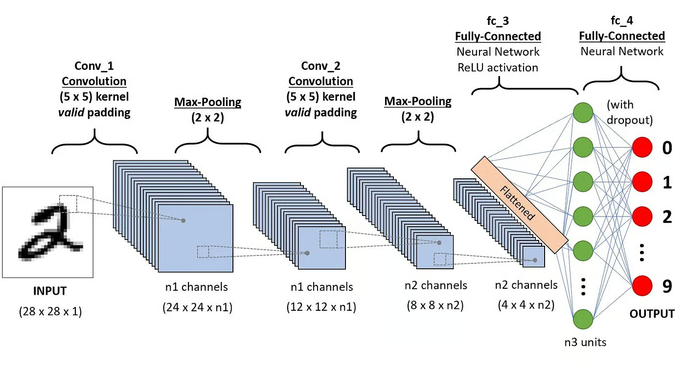
Convolution layer

The first layer of a CNN performs these convolutions, producing multiple feature maps that represent different learned filters. The weights of these filters are what the network learns during training.

Activation layer (ReLU)

After convolution, we apply a non-linearity like ReLU(x) = max(0, x). This helps the network capture complex, non-linear relationships.

Pooling layer (subsampling)

Pooling reduces spatial size by taking the maximum (Max Pooling) or average (Average Pooling) of small regions. This makes the network more efficient and invariant to small translations or distortions.

Fully connected layer

After several convolution + pooling layers, we flatten the feature maps and feed them into fully connected layers for classification or regression.

Source: DataCamp

---

5. How CNNs revolutionized image processing

CNNs changed everything because they reduced parameters drastically while preserving spatial relationships. Instead of millions of weights, a small number of shared filters capture universal visual features.

Early filters detect simple shapes. Deeper layers combine them into complex patterns. For example:

• Layer 1: Detects edges and color gradients
• Layer 2: Detects shapes like corners or textures
• Layer 3+: Detects objects like eyes, wheels, or entire faces

Example — Edge detection filter

Consider this simple filter used to detect vertical edges:

[[-1, 0, 1],
 [-1, 0, 1],
 [-1, 0, 1]]

When you convolve this filter with an image, high positive values appear wherever there’s a vertical edge. CNNs learn similar filters automatically during training but hundreds or thousands of them.

---

6. Parameter sharing & translation invariance

Unlike ANNs where every neuron has its own weights, CNN filters are shared across all spatial locations. That means the same filter scans the entire image. This parameter sharing drastically reduces complexity.

Another side effect: translation invariance. If an object moves around in the image, the CNN still detects it because the same filter applies everywhere. That’s a huge advantage over traditional ANNs.

---

7. The math intuition — why convolution works

Convolution acts like a pattern matcher. Each filter is a small matrix that highlights certain pixel arrangements. During training, backpropagation adjusts these filters to minimize the loss. Over time, filters evolve to detect features that are useful for the task maybe fur texture for cats, or circular wheels for cars.

So instead of learning “this pixel value means cat,” the CNN learns “this pattern of nearby pixels tends to appear in cats.” That’s the difference between raw memorization and feature learning.

---

8. CNN in action — a small practical example

import tensorflow as tf
from tensorflow.keras import layers, models

model = models.Sequential([
    layers.Conv2D(32, (3, 3), activation='relu', input_shape=(64, 64, 3)),
    layers.MaxPooling2D((2, 2)),
    layers.Conv2D(64, (3, 3), activation='relu'),
    layers.MaxPooling2D((2, 2)),
    layers.Flatten(),
    layers.Dense(64, activation='relu'),
    layers.Dense(10, activation='softmax')
])

model.summary()
  

This small CNN can classify 64×64 color images into 10 categories. Even though it looks simple, it’s already powerful — thanks to shared filters and local connectivity.

---

9. Comparing ANN vs CNN — the key differences

Feature	ANN	CNN
Connectivity	Fully connected — each neuron sees all inputs	Locally connected — each neuron sees a small patch
Parameters	Huge (millions)	Much smaller due to weight sharing
Spatial awareness	None	Strong — preserves pixel neighborhood structure
Translation invariance	No	Yes
Best for	Tabular, structured data	Image, video, spatial data

---

10. CNN evolution — LeNet to ResNet and beyond

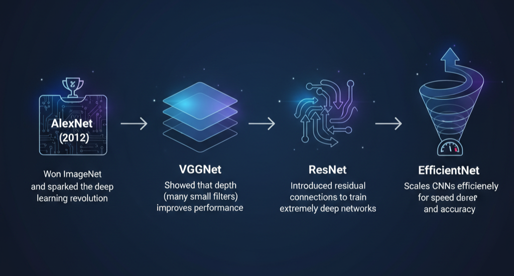
The first CNN, LeNet-5, was developed by Yann LeCun in the 1990s to read handwritten digits. It was simple — a few convolution and pooling layers — but revolutionary. Fast forward to today, and we have powerful architectures like:

• AlexNet (2012): Won ImageNet and sparked the deep learning revolution.
• VGGNet: Showed that depth (many small filters) improves performance.
• ResNet: Introduced residual connections to train extremely deep networks.
• EfficientNet: Scales CNNs efficiently for speed and accuracy.

---

11. Real-world applications of CNNs

• Facial recognition — powering phone unlock systems and surveillance.
• Medical imaging — detecting tumors or abnormalities in scans.
• Autonomous vehicles — identifying lanes, pedestrians, and obstacles.
• Art generation — neural style transfer and creative AI.
• Satellite imagery — mapping forests, cities, or weather patterns.

Basically, wherever you see an image-based AI system, there’s a CNN behind it.

---

12. Looking ahead — the next layer of understanding

CNNs aren’t perfect. They’re powerful, but they require huge datasets, and they don’t understand relationships beyond local features. That’s where newer architectures like Vision Transformers (ViTs) come in — blending the strengths of CNNs with attention mechanisms.

Still, CNNs remain the backbone of most visual AI today. Understanding them isn’t just academic — it’s foundational.

---

Final Thoughts

If ANNs were our first attempt at mimicking the brain, CNNs were our first success at mimicking the visual part of it. They taught machines to see — not by memorizing pixels, but by understanding patterns. And that shift changed everything.

---

tags: artificial neural networks, convolutional neural networks, CNN, ANN, deep learning, computer vision, image processing, receptive fields, feature maps, AlgoDecode